DeepMind X UCL | 5. Model-free Prediction

Head back to contents

This work has not been AI-generated.

Note. The notation used here might be confusing. We use $S$ to denote the state space and $S_t$ to represent the state at time $t$. Similarly, $A$ represents the action space, and $A_t$ denotes the action at time $t$.

DP

\[v_{n+1}(S_t) = \mathbb{E}^\pi \left[R_{t+1}+\gamma v_n(S_{t+1})\,|\,S_t\right]\]

What does this mean?

DP stands for Dynamic Programming. There are several different versions of DP. In this version, we improve the value function by directly evaluating the expectation on the right-hand side, i.e. the Bellman Expectation Operator. Evaluating this operator can easily become computationally infeasible when the state-action space is large. Moreover, it’s impossible to evaluate without knowledge of the environment’s dynamics. This is why we need model-free algorithms such as MC and TD.

MC

\[\begin{aligned} G_t&=R_{t+1}+\gamma G_{t+1}=\cdots=\sum_{k=0}^{T} {\gamma^k R_{t+k+1}} \text{ (target)} \\ v_{n+1}(S_t)&=v_n(S_t)+\alpha (G_t-v_n(S_t)) \text{ (update)} \end{aligned}\]

What does this mean?

MC stands for Monte Carlo. In a Monte Carlo update, the sampled return $G_t$ is determined by processing the entire $n$-th episode up to the terminal time step $T$. Then, $v_n(S_t)$ is updated towards $G_t$ with a step-size $\alpha$. Unlike DP, MC updates can be performed even without the knowledge of the rules underlying the environment, as the updates are based on samples. However, since $G_t$ can have a large variance, we use a small step-size $\alpha$ to reduce noise during updates.

TD

\[\begin{aligned} H_t&=R_{t+1}+\gamma v_t(S_{t+1})\text{ (target)} \\ v_{t+1}(S_t)&=v_t(S_t)+\alpha(H_t-v_t(S_t))\text{ (update)}\end{aligned}\]

What does this mean?

TD stands for Temporal Difference. In a Temporal Difference update, for each time step $t$ of the episode we update the value $v_t(S_t)$ to $v_{t+1}(S_t)$ by updating it towards the bootstrapped return $H_t$. We can think of TD as the sampled version of DP. TD is a bootstrapping method in the sense that it uses the estimate $v_t(S_{t+1})$ itself to create the target $H_t$. Therefore, it does not calculate the full cumulative return $G_t$. Note that the step-size $\alpha$ is also used since $H_t$ is a random variable.

Comparing MC and TD

Although the equations look similar, MC and TD differ substantially in the below aspects:

1. computation

   For a MC update, the episode needs to conclude before updating the value function, as it requires the calculation of $G_t$, which involves future terms. In contrast, TD can be updated as we go, since the target $H_t$ can be calculated for each time step.

2. bootstrapping

   In a MC update, we do not bootstrap from the value function estimate $v_n(S_t)$ to calculate the the target $G_t$, since it is independently calculated from the rewards in the time range $[t+1, T]$. However, we do bootstrap in a TD update as can be seen from the definition of the target $H_t$ - it involves the value function itself, $v_t(S_{t+1})$.

3. bias and variance

   In a MC update, the target $G_t$ is the unbiased estimator of the true value function value $v^{\pi}(S_t)$. However $G_t$ has large variance as it is the weighted sum of multiple rewards $R_k\;(k=t+1,\cdots,T)$, which are all random variables. The circumstances are different for TD updates, because the target $H_t$ only involves two random variables, $R_{t+1}$ and $v_t(S_{t+1})$. Since there are less random “components” in the target, the variance is kept low - however unbiasedness is sacrificed due to bias-variance tradeoff.

$n$-step TD

\[\begin{aligned} G_t^{(n)}&=R_{t+1}+\gamma R_{t+2}+\cdots+\gamma^{n-1}R_{t+n}+\gamma^n v_k(S_{t+n}) \text{ (target)} \\ v_{k+1}(S_t)&=v_k(S_t)+\alpha\left(G_t^{(n)}-v_k(S_t)\right)\text{ (update)}\end{aligned}\]

What does this mean?

Suppose you want to cut off the later terms in $G_t$, and bootstrap at some point instead. If we do so, we get the $n$-step TD, with $n$ reward terms ($R_{t+1},\cdots,R_{t+n}$) and one bootstrapping term ($v_k(S_{t+n})$). As expected, the $n$-step TD has intermediate bias and intermediate variance, and interpolates between MC and TD.

$\lambda$-TD

\[\begin{aligned} G_t^{\lambda}&=R_{t+1}+\gamma \left((1-\lambda)v_k(S_{t+1}) + \lambda G_{t+1}^\lambda\right) \text{ (target)} \\ v_{k+1}(S_t)&=v_k(S_t)+\alpha\left(G_t^{\lambda}-v_k(S_t)\right)\text{ (update)}\end{aligned}\]

What does this mean?

In MC, we continue sampling the rewards until the end of the episode, whereas in TD, we stop and bootstrap. We can also do something in the middle - that is, we can take a linear combination of rewards and bootstrapped value functions. This gives the $\lambda$-TD, which is another way of interpolating between MC ($\lambda=1)$ and TD ($\lambda=0$). The $\lambda$-TD can be represented as a weighted average of $n$-step returns: $G_t^\lambda=\sum_{n=1}^{T}(1-\lambda)\lambda^{n-1} G_t^{(n)}$.

$n$-step TD vs. $\lambda$-TD

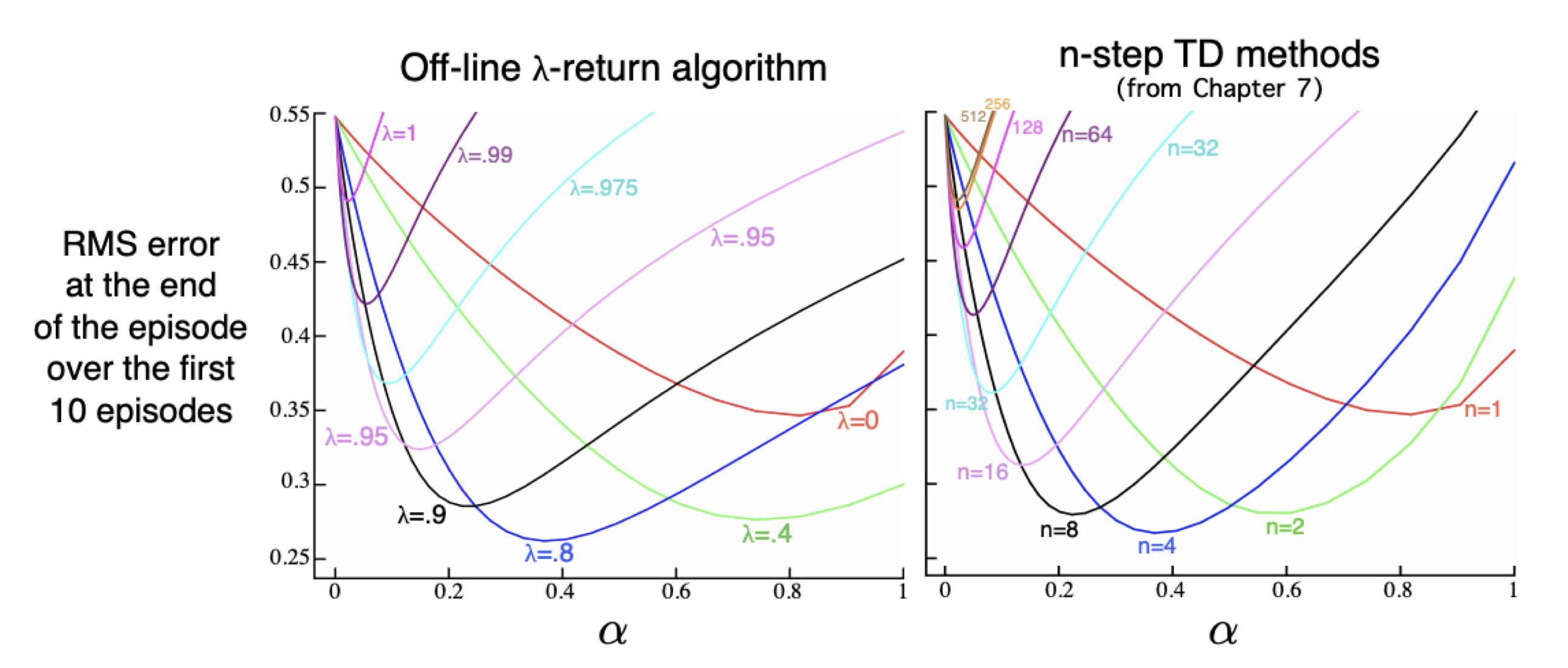
Comparing the $n$-step TD and $\lambda$-TD. The plots obtained from the $\lambda$-TD algorithm is similar to the $n$-step TD algorithm, especially when $n \approx 1/(1-\lambda)$. (Source: Deepmind X UCL Deep Reinforcement Learning Lecture 5, given by Prof. Hado van Hasselt.)

The $n$-step TD and the $\lambda$-TD are both interpolations between MC and TD, and they share commonalities. In fact, you can think of the value $1/(1-\lambda)$ as the “horizon” of the $\lambda$-TD in the sense that the $n$-step TD and $\lambda$-TD yield similar results when $n \approx 1/(1-\lambda)$. The $n$-step TD and the $\lambda$-TD both have intermediate bias and intermediate variance. Typically, intermediate values of $n$ and $\lambda$ are good as they trade off bias and variance in an appropriate way, e.g. $n=10$, $\lambda=0.9$. This gives a good starting point for training RL algorithms.

Eligibility Traces (Advanced)

Motivation: Independence of Temporal Span

In MC updates and $n$-step TD / $\lambda$-TD updates, the update depends on the temporal span of each episode. Having to wait until the end of the episode is problematic, because it prevents us from online learning (i.e., learning as new data becomes available). Can we implement MC in an online learning setup?

Prerequisite: Linear Function Approximation

The tabular value function can be written as an inner product between the one-hot feature vector $\mathbf{x}(s)$ and some weight vector $\mathbf{w}$, for any state $s$:

\[v_\mathbf{w} (s)= \mathbf{w}^{T}\mathbf{x}(s)\]

If we want to update the values for a state $s=S_t$ using MC, we update the weight acoording to the following:

\[\Delta \mathbf{w} = \alpha(G_t-v(S_t))\mathbf{x}(S_t)\]

Normally, we cannot update the values of states in the middle of the $k$-th episode. Instead, we have to update it later, simultaneously:

\[\Delta \mathbf{w}_{k+1} = \sum_{t=0}^{T-1} {\alpha (G_t-v(S_t))\mathbf{x}(S_t)}\]

But what’s interesting is that we can split the MC error $G_t-v(S_t)$ into two parts:

1. the TD error term, $\delta_t := R_{t+1}+\gamma v(S_{t+1})-v(S_t)$,
2. and the non-TD error term, $\gamma (G_{t+1}-v(S_{t+1}))$.

\[\begin{aligned} G_t-v(S_t) &= R_{t+1}+\gamma G_{t+1}-v(S_t)\\ &= R_{t+1}+\gamma G_{t+1}-v(S_t) + \gamma v(S_{t+1}) - \gamma v(S_{t+1})\\ &= (R_{t+1}+\gamma v(S_{t+1})-v(S_t)) + \gamma (G_{t+1} - v(S_{t+1})) \\ &= \delta_t+\gamma(G_{t+1} -v(S_{t+1}))\end{aligned}\]

Let’s utilize this discovery to our advantage. Note that the non-TD error term turns out to be the discounted MC error term for the next time step. Continuing the recursion, we obtain the following:

\[\begin{aligned} G_t-v(S_t) &= \delta_t+\gamma(G_{t+1} - v(S_{t+1})) \\&=\delta_t +\gamma\delta_{t+1}+\gamma^2(G_{t+2}- v(S_{t+2})) \\&= \cdots \\&=\sum_{k=t}^{T-1} {\gamma^{k-t}\delta_k} \end{aligned}\]

Now, let’s plug this into the updating equation and change the order of summation:

\[\begin{aligned} \Delta \mathbf{w}_{k+1} &= \sum_{t=0}^{T-1} {\alpha (G_t-v(S_t))\mathbf{x}(S_t)} \\ &= \sum_{t=0}^{T-1} {\alpha \left(\sum_{k=t}^{T-1} {\gamma^{k-t}\delta_k}\right)\mathbf{x}(S_t)} \\&= \sum_{k=0}^{T-1} { \alpha \delta_k\left(\sum_{t=0}^{k} {\gamma^{k-t}}\mathbf{x}(S_t)\right)} \end{aligned}\]

Defining the eligibility trace $\mathbf{e}_{k} := \sum_{t=0}^{k} {\gamma^{k-t}}\mathbf{x}(S_t)$ and renaming the summation index $k$ to $t$, we have:

\[\begin{aligned} \Delta \mathbf{w}_{k+1} &= \sum_{k=0}^{T-1} {\alpha\delta_k\mathbf{e}_k} \\ &= \sum_{t=0}^{T-1} {\alpha\delta_t\mathbf{e}_t}, \end{aligned}\]

plus the recursion relation of the eligibility trace:

\[\mathbf{e}_t=\gamma\mathbf{e}_{t-1}+\mathbf{x}_t\]

What’s “magical”, as Hado mentions in the lecture, is that the term $\alpha\delta_t\mathbf{e}_t$ now does not involve future terms at all! Therefore, we can now update the weights online, and obtain (almost) the same results as the original MC.

Even if we choose not to update the values online and instead accumulate the summation until the end of the episode, the required memory remains independent of the episode’s duration. In this case, the result will exactly equal the result of the original MC.

By altering the recursion relation as follows, we can generalize this method to the $\lambda$-TD case:

\[\tilde{\mathbf{e}}_t=\gamma\lambda\tilde{\mathbf{e}}_{t-1}+\mathbf{x}_t.\]

The derivation is similar:

\[\begin{aligned} G_t^\lambda-v(S_t) &= R_{t+1}+\gamma((1-\lambda)v(S_{t+1})+\lambda G_{t+1}^\lambda)-v(S_t)\\ &= R_{t+1}+\gamma((1-\lambda)v(S_{t+1})+\lambda G_{t+1}^\lambda)-v(S_t)+ \gamma\lambda v(S_{t+1}) - \gamma\lambda v(S_{t+1})\\ &= (R_{t+1}+\gamma v(S_{t+1})-v(S_t)) + \gamma\lambda (G_{t+1}^\lambda - v(S_{t+1})) \\ &= \delta_t+\gamma\lambda(G_{t+1}^\lambda - v(S_{t+1}))\\&=\delta_t +\gamma\lambda\delta_{t+1}+\gamma^2\lambda^2(G_{t+2}^\lambda - v(S_{t+2})) \\&= \cdots \\&=\sum_{k=t}^{T-1} {(\gamma\lambda)^{k-t}\delta_k},\\\Delta \mathbf{w}_{k+1} &= \sum_{t=0}^{T-1} {\alpha (G_t^\lambda-v(S_t))\mathbf{x}(S_t)} \\ &= \sum_{t=0}^{T-1} {\alpha \left(\sum_{k=t}^{T-1} {(\gamma\lambda)^{k-t}\delta_k}\right)\mathbf{x}(S_t)} \\&= \sum_{k=0}^{T-1} { \alpha \delta_k\left(\sum_{t=0}^{k} {(\gamma\lambda)^{k-t}}\mathbf{x}(S_t)\right)} \\&= \sum_{k=0}^{T-1} { \alpha \delta_k\tilde{\mathbf{e}}_t} \\\text{where}\\ \tilde{\mathbf{e}}_t &:= \sum_{k=t}^{T-1} {(\gamma\lambda)^{k-t}\delta_k}. \end{aligned}\]