DeepMind X UCL | 6. Model-free Control

This work has not been AI-generated.

GLIE

GLIE stands for Greedy in the Limit with Infinite Exploration. It is used to describe a set of desirable properties of a policy. GLIE is a combination of the following two properties:

Greedy in the Limit means that the policy eventually converges to a greedy policy, i.e.
\[\lim_{t \rightarrow \infty} {\pi_t(a|s)}=I(a=\operatorname{argmax}_{a' \in A}{q_t(s,a')})\]
Infinite Exploration means that all state-action pairs are explored infinitely many times, i.e.

\[\forall s, a \;\;\lim_{t\rightarrow \infty} {N_t (s,a)=\infty}\]

If we have the Infinite Exploration property, samples for each state-action pairs will accumulate enough, allowing for accurate value prediction. The Greedy in the Limit property then ensures that the policy will converge to the optimal greedy policy.

Greedy policy alone will not explore enough, and the $\epsilon$-greedy policy with fixed $\epsilon \in (0,1]$ will never fully exploit. By choosing $\epsilon$-greedy policy with $\epsilon_t=1/t$, where $t$ is the number of time-steps elapsed, we have a GLIE policy that will both explore and exploit sufficiently in the limit.

Analogy Between DP and Model-free Algorithms

In lecture 04, we covered different types of Bellman operators:

\[\begin{aligned} (T_V^\star f)(s)&=\max_{a \in A} \biggl[ {r(s, a) + \gamma \mathbb{E} \left[f(s')|s, a\right]} \bigg], \;\forall f \in V \\ (T_V^\pi f)(s)&=\mathbb{E}^\pi \bigg[ r(s, a) + \gamma f(s') \bigg| s, a \bigg], \;\forall f \in V \\(T_Q^\star f)(s,a)&=\mathbb{E} \bigg[r(s, a) + \gamma \max_{a'\in A} f(s',a') \bigg|s, a\bigg], \;\forall f \in Q \\ (T_Q^\pi f)(s, a)&=\mathbb{E}^\pi \bigg[ r(s, a) + \gamma f(s',a') \bigg| s, a \bigg], \;\forall f \in Q \end{aligned}\]

To apply a Bellman operator we need exact knowledge of the transition dynamics of the system. We can avoid this problem using a sampled version of the operator. It turns out that the sampled versions of the above Bellman operators correspond to different model-free algorithms, except for $(T_V^\star f)(s)$:

\[\begin{aligned} &(T_V^\star f)(s) \leftrightarrow \text{(None)} \\ &(T_V^\pi f)(s)\leftrightarrow \text{(TD)} \\ &\leftrightarrow v_{t+1}(S_t)=v_t(S_t)+\alpha_t\bigg(R_{t+1}+\gamma v_t(S_{t+1})-v_t(S_t)\bigg)\\&(T_Q^\star f)(s,a)\leftrightarrow \text{(Q-learning)} \\& \leftrightarrow q_{t+1}(S_t, A_t) = q_t(S_t, A_t) + \alpha_t \bigg(R_{t+1} + \gamma \max_{a' \in A}{q_t(S_{t+1}, a')-q_t(S_t, A_t)\bigg)}\\ &(T_Q^\pi f)(s, a) \leftrightarrow \text{(SARSA)} \\ &\leftrightarrow q_{t+1}(S_t, A_t) = q_t(S_t, A_t) + \alpha_t \bigg(R_{t+1} + \gamma q_t(S_{t+1}, A_{t+1})-q_t(S_t, A_t)\bigg) \end{aligned}\]

It is evident that we cannot build a sampled version of the operator $(T_V^\star f)(s)$ - Since the $\max_{a \in A}$ and the $\mathbb{E}$ operator do not commute, $(T_V^\star f)(s)$ cannot be expressed as an expectation from which we can sample upon.

SARSA is relatively simple - it’s simply the $q$-version of TD. However, Q-learning has some interesting properties that deserves attention of its own.

On & Off-Policy Learning

As humans, we learn from our experience. But we can also learn from the experience of others. In on-policy learning, the agent learns about the behavior policy $\pi$ from experience sampled from the same policy $\pi$. On the other hand, in off-policy learning, the agent learns about the target policy $\pi$ from experience sampled from a separate behavior policy $\mu$.

Using off-policy learning, we can:

learn from observing humans or other agents
re-use experience from old policies
learn about multiple policies while following one policy
learn about greedy policy while following exploratory policy

Q-Learning

Q-learning can learn the greedy policy while following any (exploratory) policy. We can see this from the update equation:

\[q_{t+1}(S_t, A_t) = q_t(S_t, A_t) + \alpha_t \bigg(R_{t+1} + \gamma \max_{a' \in A}{q_t(S_{t+1}, a')-q_t(S_t, A_t)\bigg)}\]

Here, there is no policy $\pi$ involved - you can use any behavior policy $\mu$ to converge to the optimal value function $q^\star$, as long as it is a infinite exploration policy. Once $q^\star$ is learned, we can use the (optimal) greedy policy for exploitation:

\[{\pi^\star(a|s)}=I(a=\operatorname{argmax}_{a'\in A}{q^\star(s,a')}).\]

Theorem

Q-learning converges to the optimal $q$-value function, $q\rightarrow q^\star$, as long as we take each action in each state indefinitely often AND decay the step sizes in such a way that $\sum_t\alpha_t=\infty$ and $\sum_t \alpha_t^2<\infty$.

For example,
$\alpha_t= 1/t^\omega, \omega \in (0.5, 1)$.

Overestimation in Q-Learning

In the Q-learning update equation, let’s take a look at the maximization:

\[\max_{a' \in A}{q_t(S_{t+1}, a')}\]

To write things differently:

\[\max_{a' \in A}{q_t(S_{t+1}, a')}=q_t\left(S_{t+1}, \operatorname{argmax}_{a' \in A} q_t(S_{t+1}, a')\right)\]

Suppose that the value function is currently inaccurate and has high noise. For simplicity, assume that the optimal q-value function $q^\star(S_{t+1},a’)$ stays constant regardless of the action $a’$ taken. For some of the $a’$s, the noise will add up to increase $q$. Therefore, the $\operatorname{argmax}_{a’ \in A}$ will choose the $a’$ with the highest noise value then update $q(S_{t}, A_{t})$ towards the noise-added value. Similar logic applies to the case where $q^\star(S_{t+1},a’)$ is not constant with respect to $a’$. Hence, Q-learning tends to overestimate the optimal $q$-value function.

Double Q-Learning

How can we solve this problem? We can store two action value functions, $q$ and $q’$, and alternate between the two targets below:

\[\begin{align*} \text{(target for }q \text{):}\;\;R_{t+1} + \gamma q'\left(S_{t+1}, \operatorname{argmax}_{a' \in A} q(S_{t+1},a')\right) \\\\ \text{(target for }q' \text{):}\;\;R_{t+1} + \gamma q\left(S_{t+1}, \operatorname{argmax}_{a' \in A} q'(S_{t+1},a')\right) \end{align*}\]

This eliminates the influence of noise by decoupling the selection ($\operatorname{argmax}$) step and the evaluation step.

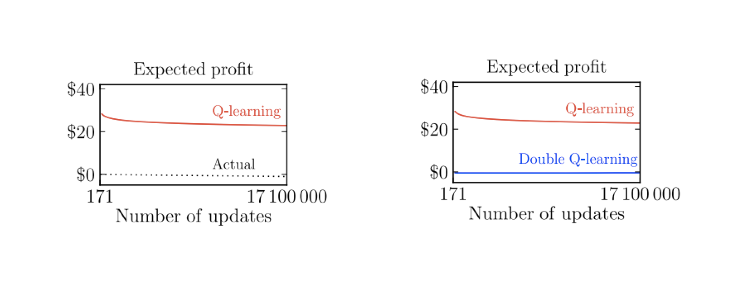
Q-learning overestimates, whereas double Q-learning does not. (Source: DeepMind X UCL Deep RL lectures)

The above plot shows how decoupling indeed eliminates the overestimation in Q-learning. We can also apply this method to SARSA whenever the behavior policy is (soft) greedy and has correlation with $q$ (we call this double SARSA).

Importance Sampling

Suppose you want to evaluate

\[\mathbb{E}_{X \sim d}[f(X)]\]

for some distribution $d$. If we sample $X$ to yield the estimate as follows,

\[\mathbb{E}_{X \sim d}[f(X)] \simeq \hat{X} :=\frac{1}{N} \sum_{i=1}^{N} f(X_i), \;\text{for each}\;X_i \sim d,\]

It could be problematic if $f(X)$ deviates significantly from $\mathbb{E}_{X \sim d}[f(X)]$ for some rare events, since it will overestimate or underestimate whenever the rare event is not sufficiently sampled.

Therefore, we can seek to sample from a different distribution $d’$ so that the rare events are sampled more. Now, suppose that we have samples $f(X_i)$ with $X_i \sim d’$. How can we evaluate the original expectation using these samples? We can first modify the original expectation as follows:

\[\begin{aligned}\mathbb{E}_{X \sim d}[f(X)]&=\sum_x d(x)f(x) \\ &= \sum_x d'(x)\frac{d(x)}{d'(x)}f(x) \\ &= \mathbb{E}_{X \sim d'} \left[\frac{d(x)}{d'(x)}f(x)\right] \end{aligned}\]

Now, we have a new expectation that can be sampled from $d’$ instead. Note that $d’$ has to be positive for all $x$ for this to work. Sampling from $d’$ gives:

\[\mathbb{E}_{X \sim d}[f(X)] \simeq \hat{X}' := \frac{1}{N} \sum_{i=1}^{N} \frac{d(X_i)}{d'(X_i)}f(X_i), \;\text{for each}\;X_i \sim d'.\]

This technique of sampling from a new distribution $d’$ to yield an estimate for the original expectation $\mathbb{E}_{X \sim d}[f(X)]$ is called Importance Sampling.

Importance Sampling for Off-Policy MC

Suppose you want to estimate the $v$-value function $v^\pi$ for some policy $\pi$ using MC, and that the trajectory $\tau_t={S_t, A_t, R_{t+1} , \cdots }$ is generated with some behavior policy $\mu$. We can get an importance sample for $G_t=G(\tau_t)=R_{t+1}+\gamma R_{t+2} + \cdots$ by reweighing the target with $\frac{p(\tau_t|\pi)}{p(\tau_t|\mu)}$ (Suppose $N=1$):

\[\frac{p(\tau_t|\pi)}{p(\tau_t|\mu)} G_t = \frac{p(A_t|S_t,\pi)p(R_{t+1},S_{t+1}|S_t,A_t)p(A_{t+1}|S_{t+1},\pi) \cdots}{p(A_t|S_t,\mu)p(R_{t+1},S_{t+1}|S_t,A_t)p(A_{t+1}|S_{t+1},\mu) \cdots} G_t\]

Luckily, the transition probability (in which most cases we do not know) cancels out and we are left with:

\[\begin{aligned}\frac{p(\tau_t|\pi)}{p(\tau_t|\mu)} G_t &= \frac{p(A_t|S_t,\pi)p(A_{t+1}|S_{t+1},\pi) \cdots}{p(A_t|S_t,\mu)p(A_{t+1}|S_{t+1},\mu) \cdots} G_t \\ &= \frac{\pi(A_t|S_t)\pi(A_{t+1}|S_{t+1}) \cdots}{\mu(A_t|S_t)\mu(A_{t+1}|S_{t+1}) \cdots} G_t \end{aligned}\]

We can then update $v^\pi$ towards the importance sampled target to get:

\[v(S_t) \leftarrow v(S_t) + \alpha\left({\frac{\pi(A_t|S_t)\pi(A_{t+1}|S_{t+1}) \cdots}{\mu(A_t|S_t)\mu(A_{t+1}|S_{t+1}) \cdots} G_t - v(S_t)} \right)\]

Importance Sampling for Off-Policy TD

Now, suppose you want to go through the same procedure with MC. In this case, you only need a single correction:

\[v(S_t) \leftarrow v(S_t) + \alpha\left(\frac{\pi(A_t|S_t)}{\mu(A_t|S_t)} (R_{t+1} +\gamma v(S_{t+1})) - v(S_t) \right)\]

The proof for this can be found in page 44 of the lecture material (link).

Expected SARSA (Generalized Q-learning)

We can also attempt to apply importance sampling to SARSA. However, we quickly realize that we don’t actually need IS because the $q$-value function conditions on selecting some action $a$. Therefore, we can simply take the expectation for the next $q$-values conditioned on policy $\pi$, while creating the trajectory according to some other policy $\mu$:

\[q(S_t, A_t) \leftarrow q(S_t, A_t) + \alpha \left(R_{t+1}+ \gamma \sum_{a \in A} \pi(a |S_{t+1})q(S_{t+1}, a)-q(S_t, A_t) \right)\]

Expected SARSA is also called Generalized Q-learning because it reduces to Q-learning when the policy chosen to be $\pi=\pi_q$, where $\pi_q$ is the greedy policy generated from $q$.