DeepMind X UCL | 7. Function Approximation

Head back to contents

This work has not been AI-generated.

Why function approximations?

It is hard to build lookup tables if the state space $S$ or the action space $A$ is large. For example, the game of go has $10^{170}$ states, which is more than the number of atoms in the universe squared. Therefore, creating the lookup table $v(s)$ is simply infeasible. Not only that, the universe itself is continuous - and we cannot give up on RL just because it is.

Therefore, we will estimate the value function using function approximation. In many cases, the function approximation will involve some parameter vector $\mathbf{w}$:

\[\begin{aligned} v_{\mathbf{w}}(s) &\approx v^\pi(s) \;(\text{or} \; v^\star(s)), \\ q_{\mathbf{w}}(s,a)&\approx q^\pi(s,a) \;(\text{or} \; q^\star(s,a)). \end{aligned}\]

The parameter vector $\mathbf{w}$ will usually be some high dimensional vector that we can adjust to approximate the the value function. In a deep RL setup, we can also imagine $v_\mathbf{w}(s)$ and $q_\mathbf{w} (s, a)$ as a neural network, a rich class of nonlinear function that maps the state space to a range of values $(v_\mathbf{w}(s):S \rightarrow \mathbb{R})$ or the state-action space to a range of values $(q_\mathbf{w}(s, a) : S \times A \rightarrow \mathbb{R})$.

Properties of RL

There are certain properties of RL we should consider when constructing function approximations for value functions. The most important of all is that the regression targets may be non-stationary because of either:

• Changing policies of the agent
  • The agent’s policy $\pi$ change $v^\pi(s)$, which then changes the target,
• Bootstrapping
  • The target involves $v^\pi(s)$ itself, which is constantly being updated,
• Non-stationary dynamics
  • There might be other learning agents in the environment,
• Previously unobserved information
  • Previously unobserved facts might influence the value function.

Tabular vs. Linear vs. Non-linear

When we use tabular function approximations, we have a good theory on how agents learn (such as the Bellman Equation). But it does not scale or generalize well to larger or continuous state-action spaces.

With linear function approximations, we have a reasonably good theory on the learning process. But the actual performance is dependent on the fixed feature mapping $\mathbf{x}:S\rightarrow \mathbb{R}^n$ (which will be discussed below).

With nonlinear function approximations (deep learning), we do not yet have a good theory at all - but we know that it works well experimentally, and that it works even better when we do not hand-engineer the feature mapping and let the neural network learn the mapping by itself.

The fact that we do not have to hand engineer features when using deep learning is quite useful, because it means that we can use it to study less well-known problems without having to worry about feature mappings.

Linear Function Approximations

Approximating state-value functions

Since we have already explored the tabular case, let’s now explore the linear case. In a linear function approximation setup, we represent the state (or the observation) at time $t$ as a vector $\mathbf{x}(S_t)$ which we will also call $\mathbf{x}_t$. This mapping $\mathbf{x}:S\rightarrow \mathbb{R}^n$ is called the feature mapping, and is considered to be fixed:

\[\begin{align*} \mathbf{x}(s)=\begin{pmatrix} x_1(s) \\ \vdots \\ x_n(s) \end{pmatrix},\; \forall s \in S. \end{align*}\]

Then we approximate the value function by a linear combination of the weights and features:

\[v_\mathbf{w}(s)=\mathbf{w}^\top \mathbf{x}(s)=\sum_{j=1}^{n} \mathbf{w}_j\mathbf{x}_j(s)\]

Approximating action-value functions

But what about action-value functions? We can use two different techniques to approximate $q(s,a)$. The first one is similar to the previous case. With the feature mapping $\mathbf{x}:S\times A \rightarrow \mathbb{R}^n$:

\[\begin{align*} \mathbf{x}(s,a)=\begin{pmatrix} x_1(s,a) \\ \vdots \\ x_n(s,a) \end{pmatrix},\; \forall s \in S. \end{align*}\]

The approximation of the value function is almost identical as before:

\[q_\mathbf{w}(s, a)=\mathbf{w}^\top\mathbf{x}(s,a)=\mathbf{w}_j\mathbf{x}_j(s,a)\]

This is called the action-in approximation because we take the action $a$ as an input of the value function. Here, we reuse the same weights $\mathbf{w}$ for different actions $a$. We also have the action-out approximation:

\[\mathbf{q}_\mathbf{w}(s)=\mathbf{W}\mathbf{x}(s),\; \text{ where }\;q_\mathbf{w}(s, a)= \mathbf{q}_\mathbf{w}(s)[a]\]

Note that $\mathbf{W}$ is a matrix. Therefore, we have different set of weights for different actions. For the action-out case we do not reuse the weights. Instead, we share the feature vector $\mathbf{x}(s)$ for all action $a$’s.

Action-in approximation is easier if the actions space is large or continuous. But for (small) discrete action spaces, action out is common. An example of this is DQN.

Objective: Minimize Loss

Now, we will construct a quadratic loss $J(\mathbf{w})$ and minimize it by optimizing our weight vector:

\[J(\mathbf{w}) = \mathbb{E}_{S \sim d} \left[(v^\pi(S)-\mathbf{w}^\top \mathbf{x}(S))^2 \right]\]

The distribution $d$ is some distribution of states in which we can sample from. Suppose we already know the value function $v^\pi(s)$. Then we can apply stochastic gradient descent (SGD) with decaying step size $\alpha_t$ to find some local minimum / saddle point of a smooth function:

\[\begin{align*} \nabla_\mathbf{w} v_\mathbf{w}(S_t)=\mathbf{x}(S_t) = \mathbf{x}_t, \\ \Delta \mathbf{w}_t = \alpha_t(v^\pi(S_t)-v_\mathbf{w}(S_t)) \mathbf{x}_t. \end{align*}\]

Note that the gradient of our value function, $\nabla_\mathbf{w} v_\mathbf{w}(S_t)$, is simply $\mathbf{x}(S_t)$. Luckily, $J(\mathbf{w})$ is quadratic in $\mathbf{w}$, and it’s Hessian is positive semi-definite everywhere in $\mathbb{R}^n$ which makes it a semi-convex(?) function. Hence, every local minimum is a global minimum. SGD with decaying step size will then ensure $J(\mathbf{w})$’s convergence to the global minimum.

MC and TD with Linear Approximation

However, we do not “know” the value function $v^\pi(S_t)$, which means we can’t use it to update our weight vector $\mathbf{w}$. Therefore, we substitute $v^\pi(s)$ with a stochastic target $G_t$:

\[\Delta \mathbf{w}_t = \alpha_t(G_t-v_\mathbf{w}(S_t)) \mathbf{x}_t.\]

This is MC with Linear Approximation. What is cool is that we can apply a supervised learning setup to the online training data

\[\{(S_0, G_0), \cdots, (S_T, G_T)\}\;\;T=\text{terminal time-step},\]

since $G_t$ is unbiased. If the variance of $G_t$ is too large, we can replace the target with the TD target $R_{t+1} + \gamma v_\mathbf{w}(S_{t+1})$ to get:

\[\Delta \mathbf{w}_t = \alpha_t(R_{t+1}+\gamma v_\mathbf{w} (S_{t+1})-v_\mathbf{w}(S_t)) \mathbf{x}_t.\]

The above update is called TD with Linear Approximation.

Convergence of MC with Linear Approximation

With linear value function approximation and suitably decaying step size $\alpha_t \rightarrow 0$, it is known that MC converges to:

\[\mathbf{w}_\text{MC} =\operatorname{argmin}_\mathbf{w} {\mathbb{E}^\pi[(G_t-v_\mathbf{w}(S_t))^2]}=\mathbb{E}^\pi [\mathbf{x}_t \mathbf{x}_t^\top]^{-1} \mathbb{E}^\pi[G_t\mathbf{x}_t]\]

We can verify this by setting the gradient of ${\mathbb{E}^\pi[(G_t-v_\mathbf{w}(S_t))^2]}$ with respect to $\mathbf{w}$ to zero:

\[\begin{align} \nabla_\mathbf{w} \mathbb{E}^\pi[(G_t - v_\mathbf{w}(S_t))^2]=\nabla_\mathbf{w} \mathbb{E}^\pi[(G_t - \mathbf{w}^\top\mathbf{x}_t)^2]&=0\\\mathbb{E}^\pi[(G_t - \mathbf{w}^\top\mathbf{x}(S_t))\nabla_\mathbf{w}(\mathbf{w}^\top\mathbf{x}_t)]&=0 \\=\mathbb{E}^\pi[(G_t - \mathbf{w}^\top\mathbf{x}_t)\mathbf{x}_t]&=0 \\= \mathbb{E}^\pi[G_t\mathbf{x}_t - \mathbf{x}_t^\top\mathbf{x}_t\mathbf{w}]&=0 \\ \mathbb{E}^\pi[\mathbf{x}_t\mathbf{x}_t^\top]\mathbf{w}=\mathbb{E}^\pi[G_t\mathbf{x}_t] \\ \mathbf{w}=\mathbf{w}_\text{MC}=\mathbb{E}^\pi[\mathbf{x}_t \mathbf{x}_t^\top]^{-1}\mathbb{E}^\pi[G_t\mathbf{x}_t]\end{align}\]

Convergence of TD with Linear Approximation

With linear value function approximation and suitably decaying step size $\alpha_t \rightarrow 0$, it is known that TD converges to:

\[\mathbf{w}_\text{TD} =\mathbb{E}^\pi [\mathbf{x}_t (\mathbf{x}_t-\gamma \mathbf{x}_{t+1})^\top]^{-1} \mathbb{E}^\pi[R_{t+1}\mathbf{x}_t]\]

We can verify this by setting the expected value of $\Delta\mathbf{w}$ to zero. Assuming $\alpha_t$ does not correlate with $R_{t+1},\mathbf{x}_t,\mathbf{x}_{t+1}$:

\[\begin{align} \mathbb{E}^\pi[\Delta \mathbf{w}]=0&=\mathbb{E}^\pi[\alpha_t(R_{t+1} + \gamma\mathbf{x}_{t+1}^\top\mathbf{w}-\mathbf{x}_t^\top\mathbf{w})\mathbf{x}_t] \\ 0 &= \mathbb{E}^\pi[\alpha_tR_{t+1} \mathbf{x}_t] + \mathbb{E}^\pi[\alpha_t\mathbf{x}_t(\gamma\mathbf{x}_{t+1}^\top-\mathbf{x}_t^\top)\mathbf{w}] \\ \mathbb{E}^\pi[\alpha_t\mathbf{x}_t(\mathbf{x}_t^\top-\gamma\mathbf{x}_{t+1}^\top)]\mathbf{w} &= \mathbb{E}^\pi[\alpha_tR_{t+1} \mathbf{x}_t] \\ \mathbf{w} = \mathbf{w}_\text{TD}&= \mathbb{E}^\pi[\alpha_t\mathbf{x}_t(\mathbf{x}_t^\top-\gamma\mathbf{x}_{t+1}^\top)]^{-1} \mathbb{E}^\pi[R_{t+1} \mathbf{x}_t]\end{align}\]

This differs from the MC solution. Remember, TD updates have less variance but may be biased. But since they have less variance, they tend to converge faster.

Residual Bellman updates

Note that the TD update is not a gradient update, since it ignores the dependence of $v_\mathbf{w}(S_{t+1})$ on $\mathbf{w}$.

\[\Delta \mathbf{w}_t = \alpha \delta \nabla_\mathbf{w} v_\mathbf{w}(S_t)\;\text{ where }\; \delta_t= R_{t+1} + \gamma v_\mathbf{w}(S_{t+1})-v_\mathbf{w}(S_t)\]

To remedy this, we can use the Bellman residual gradient update, where the Bellman loss is given as $\mathbb{E}^\pi[\delta_t^2]$ and we take the gradient of it to update $\mathbf{w}$:

\[\nabla_\mathbf{w}\mathbb{E}^\pi[\delta_t^2]=\mathbb{E}^\pi[\nabla_\mathbf{w}(\delta_t^2)]=2\mathbb{E}^\pi[\delta_t \nabla_\mathbf{w}\delta_t]\] \[\Delta \mathbf{w}_t = \alpha\delta_t \nabla_\mathbf{w}\delta_t = \alpha \delta_t \nabla_\mathbf{w} (v_\mathbf{w}(S_t)-\gamma v_\mathbf{w}(s_{t+1}))\]

However, residual Bellman updates tend to work worse in practice.

The Deadly Triad

Algorithms that combine:

• Bootstrapping
• Off-policy learning, and
• Function approximation

may diverge. This is called the deadly triad. However, just because an algorithm combines the three methods does not mean that it is divergent - rather, we cannot guarantee the convergence of an algorithm if is has combined the above three.

Summary

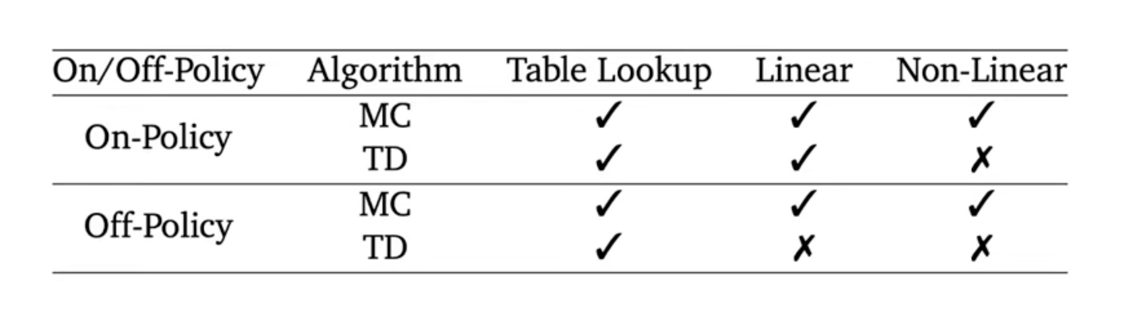
In addition to the deadly triad, we cannot guarantee the convergence of MC or TD when we combine on-policy learning with bootstrapping and non-linear function approximation. In summary, the deadly triad is the theoretical risk due to combinations of different methods in reinforcement learning, but is rarely seen in practice.