Introduction to Deep Learning
한국어 버전 보기 / View Korean Version
This work has not been AI-generated.
This is a 14-day comprehensive course for learning the fundamentals of deep learning.
Week 1
Goal of the week
A basic walkthrough of linear algebra and python
Day 1 (1/8)
CH1 | Vectors
Prob 1.1
(a) Explain what vectors are in 3-4 sentences, using the terms below:
Vector addition, scalar multiplication, arrow, list of numbers.
(b) Explain what a zero-vector is, then explain the difference between the zero vector $\mathbf{0}$ and the scalar $0$.
Note. A vector is denoted by either a boldface letter, or a letter with an arrow on top. ex) $\mathbf{v}, \vec{v}$
Vector addition, scalar multiplication, arrow, list of numbers.
(b) Explain what a zero-vector is, then explain the difference between the zero vector $\mathbf{0}$ and the scalar $0$.
Note. A vector is denoted by either a boldface letter, or a letter with an arrow on top. ex) $\mathbf{v}, \vec{v}$
Prob 1.2
If $n$ is a positive integer, then an ordered $n$-tuple is a sequence of $n$ real numbers $(v_1, v_2, …, v_n)$. The set of all ordered $n$-tuples is called $n$-space and is denoted by $R^n$. - Contemporary Linear Algebra, Howard Anton & Robert C. Busby, p.7.
$\mathbf{v}=\begin{bmatrix} x_1 \newline x_2 \end{bmatrix}$is an element of the $n$-space, that is, $\mathbf{v} \in \mathbb{R}^n$. What is $n$?
Note.
- It does not matter whether the vectors are written vertically or horizontally at this stage. We also do not care about how the brackets look like, i.e., $[\cdot], (\cdot)$ are the same.
- $R$(or $\mathbb{R}$) denotes the set of real numbers. Do not be confused with other sets, such as $N$(or $\mathbb{N}$), $Z$(or $\mathbb{Z}$) or $C$(or $\mathbb{C}$).
- We can denote the $n$-space by $R^n$(as in the book) or by $\mathbb{R}^n$(as in the problem). You may use either notation.
- We simply read $\mathbf{v} \in \mathbb{R}^n$ as “v in R n”, or “v is in R n” depending on the context.
Vocab. integer = 정수, tuple = 순서쌍, real number = 실수, space = 공간, element = 원소
Prob 1.3
Give an example for each arithmetic rule (a) through (g), using $2$-tuples.
If $\mathbf{u}$, $\mathbf{v}$, and $\mathbf{w}$ are vectors in $R^n$, and if $k$ and $l$ are scalars, then:
(a) $\mathbf{u}+\mathbf{v}=\mathbf{v}+\mathbf{u}$
(b) $(\mathbf{u}+\mathbf{v})+\mathbf{w}=\mathbf{u}+(\mathbf{v}+\mathbf{w})$
(c) $\mathbf{u}+\mathbf{0}=\mathbf{0}+\mathbf{u}=\mathbf{u}$
(d) $\mathbf{u}+(-\mathbf{u})=0$
(e) $(k+l)\mathbf{u}=k\mathbf{u}+l\mathbf{u}$
(f) $k(\mathbf{u}+\mathbf{v})=k\mathbf{u}+k\mathbf{v}$
(g) $k(l\mathbf{u})=(kl)\mathbf{u}$
(h) $1\mathbf{u}=\mathbf{u}$
- Contemporary Linear Algebra, Howard Anton & Robert C. Busby, p.9.
Vocab. zero-vector = 영벡터, scalar = 스칼라, arithmetic rule = 연산규칙.
Solution for (a).
(a) $(1, 0) + (2, 2) = (2, 2) + (1, 0) = (3, 3)$
Prob 1.4
$\mathbf{x}= (x_1, x_2)\in \mathbb{R}^2$ is a 2-dimensional vector. find the set of $\mathbf{x}$ satisfying the below equation by filling in the blank.
\[\begin{align*} & 3x_1+x_2=0 \newline & \textrm{Solution: } \{(t, \Box t) | t \in \mathbb{R} \} \end{align*}\]Vocab. 2-dimensional vector = 이차원 벡터, satisfy = 만족하다.
Prob 1.5
Solve the below exercises from the book Contemporary Linear Algebra.
Exercise 11. Let $\mathbf{u}=(-3,1,2,4,4)$, $\;\mathbf{v}=(4,0,-8,1,2)$, and $\mathbf{w}=(6,-1,-4,3,-5)$. Find the components of
(a) $\mathbf{v}-\mathbf{w}$
(b) $6\mathbf{u}+2\mathbf{v}$
(c) $(2\mathbf{v}-7\mathbf{w})-(8\mathbf{v}+\mathbf{u})$
- Contemporary Linear Algebra, Howard Anton & Robert C. Busby, p.13.
Exercise 13. Let $\mathbf{u}$, $\mathbf{v}$ and $\mathbf{w}$ be the vectors in Exercise 11. Find the components of the vector $\mathbf{x}$ that satisfies the equation $2\mathbf{u}-\mathbf{v}+\mathbf{x}=7\mathbf{x}+\mathbf{w}$. - Contemporary Linear Algebra, Howard Anton & Robert C. Busby, same page as above.
Solution.
Exercise 11.
(a) $\mathbf{v}-\mathbf{w}=(-2,1,-4,-2,7)$
(b) $6\mathbf{u}+2\mathbf{v}=(-10,6,-4,26,28)$
(c) $(2\mathbf{v}-7\mathbf{w})-(8\mathbf{v}+\mathbf{u})=(-77,8,94,-25,23)$
- Contemporary Linear Algebra, Howard Anton & Robert C. Busby, p.A9.
Exercise 13.
$\mathbf{x}=(-\frac{8}{3},\frac{1}{2},\frac{8}{3}, \frac{2}{3}, \frac{11}{6})$
- Contemporary Linear Algebra, Howard Anton & Robert C. Busby, same page as above.
Vocab. component=성분.
Prob 1.6
Find examples of (a) a pair of two parallel vectors, and (b) a pair of two orthogonal vectors in $\mathbb{R}^2$(the xy-plane).
Vocab. parallel=평행한, orthogonal=수직인.
CH2 | Linear combinations, span, and basis vectors
Prob 2.1
Linear combination, span, and linear independence.
(a) Give an example of a linear combination of three vectors in $\mathbb{R^2}$. Are these three vectors linearly independent?
(b) What is the difference between (i) a linear combination of three vectors and (ii) the span of three vectors? Answer the question using the mathematical term : set.
(c) What is linear independence? Give an example of a linearly independent set of vectors in $\mathbb{R}^4$.
(d) Answer the quiz at the end of the video.
Note. linear combination = 선형 결합. span = 스팬. linearly independent = 선형 독립. set = 집합.
Prob 2.2
\[\begin{align*} & 3x_1 + 2x_2 - x_3 = 0 \newline & 6x_1 + 4x_2 - 2x_3 = 0 \newline & -3x_1 -2x_2 +x_3 = 0 \end{align*}\](a) Solve for the set of vectors $\mathbf{v}=\begin{bmatrix} x_1 \newline x_2 \newline x_3 \end{bmatrix} \in \mathbb{R}^3$ which satisfies the system of equations shown above.
(b) Express $\mathbf{v}$ as a linear combination of two linearly independent vectors.
Vocab. system of equations = 연립방정식.
Day 2 (1/9)
CH3 | Linear transformations and matrices
Prob 3.1
Basic concepts of linear transformations.
(a) What are transformations? What are linear transformations?
(b) Suppose the matrix $A=\begin{bmatrix}1 & 2 \newline 3 & 4 \end{bmatrix}$ represents a linear transformation from $\mathbb{R}^2$ to $\mathbb{R}^2$. Where do the two canonical basis vectors $\mathbf{i}=\begin{bmatrix} 1 \newline 0 \end{bmatrix}$ and $\mathbf{j} = \begin{bmatrix} 0 \newline 1 \end{bmatrix}$ map to?
(c) Where do the vectors $\mathbf{v}=\begin{bmatrix} 2 \newline 3 \end{bmatrix}$ and $\mathbf{w} = \begin{bmatrix} -1 \newline 2 \end{bmatrix}$ map to? Explain your answers.
(d) Answer (b), (c) in the case where the matrix $A$ is replaced by the matrix $B=\begin{bmatrix}-1 & 2 \newline 2 & -4 \end{bmatrix}$.
Note. Matrices are usually denoted by capital letters. In some cases, we will use boldface capital letters too.
Vocab. transformation = 변환, linear transformation = 선형 변환, canonical = 기본의, matrix = 행렬.
Prob 3.2
The formal definition of linear transformations. At the end of the second video, the formal definition of linear transformations is introduced.
(a) State the formal definition, and
(b) show that the transformation $L_A(\mathbf{x})=A\mathbf{x}$ defined by multiplying the matrix $A$ on the left side of the vector $\mathbf{x} \in \mathbb{R}^2$, is in fact linear.
In other words, show that $L_A$ fits the formal definition of a linear transformation defined in (a).
Note. refer to the matrix-vector multiplication rule below.
\[\begin{align*} A\mathbf{x}=\begin{bmatrix} a & b \newline c & d\end{bmatrix} \begin{bmatrix} x \newline y\end{bmatrix} = x\begin{bmatrix} a \newline c\end{bmatrix} + y\begin{bmatrix} b \newline d\end{bmatrix} = \begin{bmatrix} ax+by \newline cx+dy\end{bmatrix} \end{align*}\]Vocab. transformation = 변환, linear transformation = 선형 변환, canonical = 기본의, matrix = 행렬.
Prob 3.3
Practicing matrix-vector multiplication. Using the matrix-vector multiplication rule in Prob 3.2, reduce the following matrix-vector products into a single vector (fill in the ?s) :
(a) $A\mathbf{x}=\begin{bmatrix} 1 & 3 \newline 5 & -3\end{bmatrix} \begin{bmatrix} 2 \newline 1\end{bmatrix}= \begin{bmatrix} ? \newline ?\end{bmatrix}$
(b) $B\mathbf{y}=\begin{bmatrix} -3 & -1 \newline 2 & 2\end{bmatrix} \begin{bmatrix} -1 \newline 1\end{bmatrix}= \begin{bmatrix} ? \newline ?\end{bmatrix}$
Now, (c) extend the definition of the matrix-vector multiplication into higher dimensions. In other words, find the analogous formula for calculating matrix-vector products for $3 \times 3$ matrices and $3$-tuples(vectors). You can do this for $n \times n$ matrices and $n$-tuples(vectors), for any $n$. Did you find it?
Then, using the formula you have found, calculate the following matrix-vector multiplication:
(d) $C\mathbf{v}=\begin{bmatrix} 1 & 3 & -1 \newline 5 & -3 & 1 \newline 2 & 1 & -2\end{bmatrix} \begin{bmatrix} 2 \newline 1 \newline 2\end{bmatrix}= \begin{bmatrix} ? \newline ? \newline ?\end{bmatrix}$
(e) $D\mathbf{w}=\begin{bmatrix} -3 & -1 & 4 \newline 2 & 2 & -1 \newline 3 & -1 & 3\end{bmatrix} \begin{bmatrix} -1 \newline 1 \newline 3\end{bmatrix}= \begin{bmatrix} ? \newline ? \newline ?\end{bmatrix}$
Vocab. product = 곱, dimension = 차원, analogous = 대응되는·비슷한.
Day 3 (1/10)
CH4 | Matrix multiplication as composition
Prob 4.1
Composition of matrices. In the video, we have learned how applying two $2 \times 2$ matrices $M_1$ and $M_2$ consecutively to the basis vectors $\mathbf{i}$ and $\mathbf{j}$ gives the columns of the product matrix $M_2 M_1$. For example, applying the rotation $M_1= \begin{bmatrix} 0 & -1 \newline 1 & 0 \end{bmatrix}$ and then the shear $M_2= \begin{bmatrix} 1 & 1 \newline 0 & 1 \end{bmatrix}$to the vector $\mathbf{i}= \begin{bmatrix} 1 \newline 0 \end{bmatrix}$ gives $\begin{bmatrix} 1 \newline 1 \end{bmatrix}$, which is the first column of the matrix $M_2 M_1$.
Note. The ordering of the multiplication is from right to left, in the same way we compose functions, $(g \circ f)(x)=g(f(x))$.
(a) Explain how the elements of the matrix $M_2 M_1$ is determined, and extend the result to $3 \times 3$ matrices. In other words, find the matrix-matrix multiplication formula for $3 \times 3$ (and possibly, $n\times n$) matrices.
You may refer to the $2\times2$ matrix-matrix multiplication formula below:
\[\begin{align*} \begin{bmatrix}a & b \newline c & d \end{bmatrix} \begin{bmatrix}e & f \newline g & h \end{bmatrix} = \begin{bmatrix}ae+bg & af+bh \newline ce+dg & cf+dh \end{bmatrix} \end{align*}\](b) Give an instance of the formula found in (a), i.e. plug in actual numbers so that you can practice the calculation process yourself. You may use the matrices $C$ and $D$ in prob 3.3-(d),(e). Make sure that the matrices each have at least $6$ non-zero elements, so that the calculations are not too easy.
Vocab. composition = 합성, consecutively = 연이어서, column = 열, rotation = 회전, shear = 전단, instance = 예시·사례.
Prob 4.2
Expressing the matrix-matrix product formula using the sigma notation. When you calculate matrix-matrix products, it is easier if you visualize it as taking the sum-of-product of rows and columns. Notice how the number of columns (or the width) of the matrix $A$ must match the number of rows (or the height) of the matrix $B$.
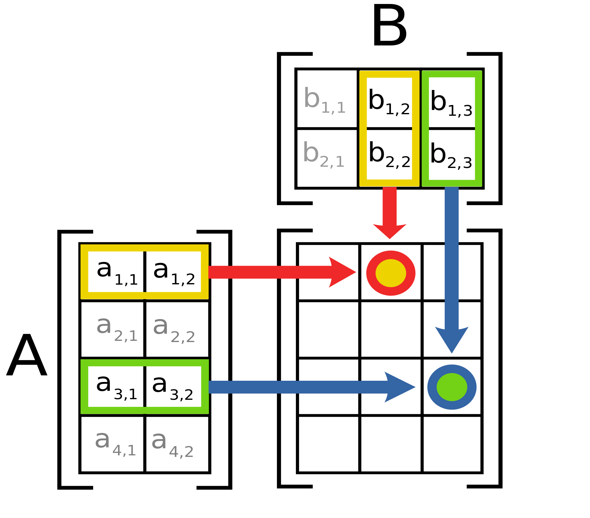
Source : Matrix Multiplication, Wikipedia
(a) Visualize (draw) your computation procedures in prob 3.3 as in the above image.
(b) Visually check that the $2\times2$ matrix-matrix multiplication formula in prob 4.1-(a) is correct.
(c) When we calculate $(AB)_{ij}$, the $i$-th row, $j$-th column element of the matrix $AB$, we calculate the sum-of-products as in below:
\[(AB)_{ij}=a_{i1}b_{1j}+a_{i2}b_{2j}\]You can verify this by plugging in $i=1$ and $j=2$ and checking if it gives the value at the yellow dot. (Or alternatively, $i=3$ and $j=3$ and checking if it yields the green dot).
Since this is a sum-of-products, we can express $(AB)_{ij}$ using the the sigma notation, i.e.,
\[(AB)_{ij}=a_{i1}b_{1j}+a_{i2}b_{2j}=\sum_{k=1}^{2}a_{ik}b_{kj}.\]Question. How would you extend this idea to multiplying any $m \times s$ matrix $A$ and $s \times n$ matrix $B$? Put in another way, express the matrix-matrix product formula using the sigma notation.
Hint. Fill in the blanks:
\[(AB)_{ij}=a_{i1}b_{1j}+a_{i2}b_{2j}+ \cdots + +a_{is}b_{sj}=\sum_{k=\Box}^{\Box}a_{i\Box}b_{\Box j}.\]Note.
- The commas between the indices $i$ and $j$ are removed for simplicity.
- Keep in mind that the indices $i$ and $j$ are different from the basis vectors $\mathbf{i}$ and $\mathbf{j}$, which we have been discussing beforehand.
- When we say that a matrix is $m \times n$, it means that the height of the matrix is $m$ and the width of the matrix is $n$. Therefore, the order matters.
- indices is the plural of index.
Vocab. visualize = 시각화하다, procedure = 과정, row = 행, column = 열, extend = 확장·일반화하다, index = 번째수.
Prob 4.3
The transpose of a matrix, row vectors, column vectors, and the length of a vector. The transpose of an $m \times n$ matrix $A$ is simply the matrix $A$ flipped along the diagonal, and is denoted by $A^T$. You may also think of this as interchanging the rows and columns of the matrix.
As an example, in the case where $A=\begin{bmatrix}1 & 2 & 3 \newline 4 & 5 & 6 \end{bmatrix}$, the transpose of $A$ or $A^T=\begin{bmatrix} 1 & 4 \newline 2 & 5 \newline 3 & 6 \end{bmatrix}$.
Also, viewing the $n$-dimensional vector $\mathbf{x}$ as an $n \times 1$ matrix, we can consider its transpose too. For example, given the vector $\mathbf{x}=\begin{bmatrix} 1 \newline 2 \newline 3 \end{bmatrix}$, the transpose of $\mathbf{x}$ or $\mathbf{x}^T=\begin{bmatrix} 1 & 2 & 3 \end{bmatrix}$.
We will now distinguish these two types of vectors as column vectors and row vectors.
Lastly, the dot product of two vectors $\mathbf{x, y} \in \mathbb{R}^n$ is denoted by $\mathbf{x} \cdot \mathbf{y}$ and is defined as follows:
\[\begin{align*} \mathbf{x} \cdot \mathbf{y} = \mathbf{x}^T \mathbf{y} = \begin{bmatrix} x_1 & x_2 & \cdots & x_n \end{bmatrix} \begin{bmatrix} y_1 \newline y_2 \newline \vdots \newline y_n \end{bmatrix} =x_1y_1+x_2y_2+ \cdots + x_ny_n = \sum_{k=1}^{n} x_k y_k. \end{align*}\]Now, consider the following:
(a) Express the matrix vector product using the dot product. More specifically, let $\mathbf{r}{i}(A)$ be the $i$-th row vector of the matrix $A$ and $\mathbf{c}{j}(B)$ be the $j$-th column vector of the matrix $B$. What is $(AB)_{ij}$, the $i$-th row, $j$-th column element of the matrix $AB$?
(b) If the transpose of an $m\times n$ matrix $A$ is equal to itself, or $A=A^T$, what must be the relation between $m$ and $n$? (When $A=A^T$, $A$ is called a symmetric matrix.)
(c) A $2 \times 2$ matrix $I$ maps every vector in $\mathbb{R}^2$ to itself. Find $I$, and show that $I$ is symmetric.
(d) Prove $\mathbf{x} \cdot \mathbf{x} \ge 0$ for any $\mathbf{x}=[x_1, x_2, \cdots, x_n]^T \in \mathbb{R}^n$, then prove that $\mathbf{x} \cdot \mathbf{x}=0$ if and only if $\mathbf{x} =\mathbf{0}$. Remark. Since we have proven this fact, we can naturally define the length of a vector $\mathbf{x}$ as $\lVert\mathbf{x}\rVert=\sqrt{\mathbf{x} \cdot \mathbf{x}}=\sqrt{x_1^2+x_2^2+ \cdots x_n^2}$. If there exists a vector $\mathbf{x}$ such that $\mathbf{x} \cdot \mathbf{x}<0$, the inside of the square root will become negative, which would be a total disaster!
Note. $[x_1, x_2, \cdots, x_n]^T$ is a column vector with components $x_1, x_2, \cdots,x_n$. Keep the definition of transposition in mind.
Vocab. transpose = 전치, transpose of a matrix = 전치행렬, column vector = 열벡터, row vector = 행벡터, dot product = 점곱, symmetric matrix = 대칭행렬.
Prob 4.4 (HARD)
Associative, non-commutative, and distributive property of matrices.
(a) Prove that the matrix multiplication is associative for $2\times2$ matrices, using only the matrix-matrix multiplication formula.
Refer to the $2\times2$ matrix-matrix multiplication formula, or alternatively, you may use the same formula expressed in sigma notation, which are all given below:
\[\begin{align*} \begin{bmatrix}a & b \newline c & d \end{bmatrix} \begin{bmatrix}e & f \newline g & h \end{bmatrix} = \begin{bmatrix}ae+bg & af+bh \newline ce+dg & cf+dh \end{bmatrix} \newline \textrm{or} \newline (AB)_{ij}=\sum_{k=1}^{s}a_{ik}b_{kj},\; s=2. \end{align*}\]Note. Although we have proved the associativity of matrix multiplication in the video visually, it is better if we can prove this concretely using the multiplication formula.
(b) Give an example of two matrices which are non-commutative (with respect to the matrix multiplication operation), other than the one presented in the video. Can you find two matrices that commute with each other?
(c) Prove that the matrix multiplication is distributive over matrix addition for $2 \times 2$ matrices, using the matrix-matrix multiplication formula and the matrix addition formula. i.e., show the following:
\[\begin{align*} & A(B+C)=AB+AC, \newline & \textrm{for } A=\begin{bmatrix} a_{11} & a_{12} \newline a_{21} & a_{22}\end{bmatrix}, B=\begin{bmatrix} b_{11} & b_{12} \newline b_{21} & b_{22}\end{bmatrix}, C=\begin{bmatrix} c_{11} & c_{12} \newline c_{21} & c_{22}\end{bmatrix}. \end{align*}\]Refer to the $2\times2$ matrix-matrix multiplication formula in problem (a) and the $2\times2$ matrix addition formula. Alternatively, you may use the matrix addition formula expressed in terms of each element, which are all given below:
\[\begin{align*} & \begin{bmatrix}a & b \newline c & d \end{bmatrix}+\begin{bmatrix}e & f \newline g & h \end{bmatrix} = \begin{bmatrix}a+e & b+f \newline c+g & d+h \end{bmatrix} \newline & \textrm{or } \newline (A+B)_{ij} = a_{ij} + b_{ij} \end{align*}\](d) What does the matrix-matrix multiplication & addition formula mean, in a visual context? Explain for each case.
Vocab. associative = 결합법칙이 성립하는, commutative = 교환법칙이 성립하는, distributive = 분배법칙이 성립하는, concretely = 확실하게, commute with each other = 서로 교환 가능하다(=연산 순서를 바꿔도 변하지 않는다), in terms of ~ = ~에 대해.
Day 4-5 (1/11-1/12)
💡 SKIP - 인후 요청
Day 6 (1/13)
CH5 | Three-dimensional linear transformations
https://www.youtube.com/watch?v=rHLEWRxRGiM&list=PLZHQObOWTQDPD3MizzM2xVFitgF8hE_ab&index=5
Prob 5.1
(a) Explain how the three dimensional linear transformation works in your own words.
(b) How would you visualize higher-order linear transformations? (Or, is it better not to?)
Prob 5.2
A rotation (which is a linear transformation) maps the basis vectors $\mathbf{i}=[1\;\;0\;\;0]^T, \;\mathbf{j}=[0\;\;1\;\;0]^T, \;\mathbf{k}=[0\;\;0\;\;1]^T$ to the vectors $\mathbf{j}=[0\;\;1\;\;0]^T, \;\mathbf{k}=[0\;\;0\;\;1]^T, \;\mathbf{i}=[1\;\;0\;\;0]^T$, respectively.
(a) Find the matrix $P$ representing the $3$-dimensional rotation.
(b) Find the axis of rotation and the rotation angle.
Prob 5.3
Linear transformation from $\mathbb{R}^n$ to $\mathbb{R}^m$. Now, consider a linear transformation from $\mathbb{R}^2$ to $\mathbb{R}^3$. This would be represented by a $3 \times 2$ matrix, such as the one below:
\[\begin{align*} W=\begin{bmatrix} -3 & -1 \newline 2 & 2 \newline 3 & -1\end{bmatrix}\in\mathbb{R}^{3\times2}. \end{align*}\]Note. $\mathbb{R}^{m\times n}$ denotes the set of all $m \times n$ matrices. Notice how the input $\mathbf{x}=\begin{bmatrix} x_1 \newline x_2 \end{bmatrix} \in \mathbb{R}^2$ is mapped to $W\mathbf{x}=x_1\begin{bmatrix} -3 \newline 2 \newline 3 \end{bmatrix} + x_2\begin{bmatrix} -1 \newline 2 \newline 1 \end{bmatrix}\in\mathbb{R}^3$.
(a) From what we’ve learned, we can say that $W\mathbf{x}$ is a linear combination of $[-3 \;\; 2 \;\; 3 ]^T$ and $[-1 \;\; 2 \;\; 1]^T$. If $\mathbf{x}$ moves around all of $\mathbb{R}^2$, where does $W\mathbf{x}$ move around in $\mathbb{R}^3$? Determine the shape of the set given below:
\[\textrm{Im}(L_W)=\left\{W\mathbf{x}\;|\;\mathbf{x} \in \mathbb{R}^2\right\} \subset \mathbb{R}^3.\]Note. The set is called the image of $L_W$, where $L_W$ denotes the linear transformation given by the matrix $W$. It is also called the range of $L_W$.
(b) Can you find a point in $\mathbb{R}^3$ where $W\mathbf{x}$ cannot reach? Find a point in $\mathbb{R}^3$ that lies outside of $\textrm{Im}(L_W)$.
(c) Suppose $W$ is replaced by $W’=\begin{bmatrix} 3 & -1 \newline -6 & 2 \newline 3 & -1\end{bmatrix}.$ What happens to the shape of $\textrm{Im}(L_W)$?
(d) State all possible shapes of $\textrm{Im}(L_M)$ for $M \in \mathbb{R}^{3 \times 2}$, and the corresponding conditions of $M$ for each shape. Can $\textrm{Im}(L_M)$ be equal to $\mathbb{R}^3$?
(e) Solve (a), (b), (c) for $W^T=\begin{bmatrix} -3 & 2 & 3 \newline -1 & 2 & -1 \end{bmatrix}$ , $(W’)^T=\begin{bmatrix} 3 & -6 & 3 \newline -1 & 2 & -1\end{bmatrix}$. How are the circumstances different?
(f) Solve (d) with $M \in \mathbb{R}^{2 \times 3}$ instead of $M \in \mathbb{R}^{3 \times 2}$. Can $\textrm{Im}(L_M)$ be equal to $\mathbb{R}^2$?
Vocab. image = 상, range = 치역, circumstance = 상황.
Day 7 (1/14)

Starting Python…
For Python Newbies
Part 1 | Lecture
- Walk through the basic concepts of Python, using the above Python tutorial.
- The tutorial consists of 18 videos, with a total lecture time of 90 minutes. Keep in mind that you will need to pause the video from time to time, so expect more than 90 minutes for completing Part 1.
Part 2 | Problem Solving
- Sign up for the above website.
- Head over to 문제 → 문제집 → Python 기초 100제.
- Solve the even-numbered exercises 6002~6046, EXCEPT 6028 and 6046.
- You’ll be solving a total of 21 questions. Each exercise is simple enough, so it won’t take more than 5 minutes to solve. Expect a total of 105 minutes for completing Part 2.
- If an exercise does take more than 5 minutes, skip it and move on to the next one. Record the ones you have skipped.
For Python Beginners & Amateurs
- Skip Part 1. In Part 2, You may choose whichever exercise to solve, but solve at least 15 exercises. Solve the ones that seems the most difficult to you. If you have time left, head over to Day 8.
For Professionals:
- Skip this content, proceed from day 10.
Day 8 (1/15)
For Python Newbies
Part 1. Lecture
- Learn how to use if statements, while & for loops.
- The above control statement tutorial consists of 11 videos, with a total lecture time of 48 minutes. Again, keep in mind that you’ll need to pause the video occasionally to practice the code yourself.
Part 2. Problem Solving
- Head over to 문제 → 문제집 → Python 기초 100제, or use the above link.
- Solve the even-numbered exercises 6048~6094, EXCEPT 6082.
- You’ll be solving a total of 23 questions. Skip whenever it takes more than 15 minutes to complete the exercise. Record the ones you have skipped. If you’re running out of time, you may skip the exercises with lower-than-50% success rates.
For Python Beginners & Amateurs
- Skip Part 1. In Part 2, (as in before) you may choose whichever exercise to solve. Solve all difficult (success rate < 40%) exercises. Some of the exercises can take more than 30 minutes to solve. If you have time left, you can head over to Day 10.
For professionals
- Skip the content. Proceed from Day 10.
Day 9 (1/16)
💡 SKIP - Dad’s birthday! 🥳
Day 10 (1/17)
Notice
We’re going to go through the very basics of deep learning, first without code.
(In other words, we will be skipping Python, for now. We’ll get back to Python after we finish the video course on deep learning.)
CH1 | But what is a neural network?
https://www.youtube.com/watch?v=aircAruvnKk
Prob 1.1
(a) What is the naive definition of a neuron?
(b) Explain the role of matrix multiplication in neural networks.
(c) Describe the full definition of a neuron using the following term: function.
(d) Give the formula for each function and draw them: $y=\sigma(x), \; y=\textrm{ReLU}(x).$ Which function would be simpler to evaluate (on a computer)?
(e) What are layers? Explain what layers are, based on the definition of a neuron.
Prob 1.2
Expand the following expression in terms of each element.
\[\mathbf{a}^{(1)}=\sigma(W\mathbf{a}^{(0)}+\mathbf{b})\]Day 11 (1/18)
CH2 | Gradient descent, how neural networks learn
https://www.youtube.com/watch?v=IHZwWFHWa-w
Prob 2.1
(a) In the video, what does the training data consist of?
Note. The setup used in the digit-classifier example is called a “supervised learning” setup, in the sense that the neural network is under the supervision of the data-label pair (which are made by humans). There’s also the “unsupervised learning” setup, where the neural network is forced to pick up underlying patterns from the unlabeled data.
(b) What is the role of the cost function?
Note. The cost function has alternative names - it is also called the “loss function”, or the “objective function”.
Prob 2.2
(a) Explain how the gradient descent works in 1D (if it has only $1$ parameter). If the cost function is denoted $C(x)$ (with $x$ being its only parameter), and $\frac{dC}{dx}(x)>0$, how should you update the parameter $x$ for $C(x)$ to decrease? Assume that the updating step is small.
(b) Explain how the gradient descent works in 2D (if it has $2$ parameters). If the cost function is denoted $C(x, y)$ (with $x$ and $y$ being its parameters), and $\nabla C(x,y)=(1,2)$, how should you update the parameters $x$ and $y$ for $C(x, y)$ to decrease? Assume that the updating step is small.
(c) How would the gradient descent work in $n$-dimensions, i.e. if it has $n$ parameters? Would it work the same as in (a) and (b)?
Prob 2.3
(a) Explain the two concepts ① local minimum and ② global minimum, respectively.
(b) Suppose the gradient descent on the cost function $C$ has been executed multiple times, and the parameters $\mathbf{p}=(p_1, p_2, \cdots, p_n)$ have converged to a single point $\mathbf{p}^{(\infty)}$. Can we be sure that $\mathbf{p}^{(\infty)}$ is a global minimum of the cost function $C$?
Day 12 (1/19)
CH3 | What is backpropagation really doing?
https://www.youtube.com/watch?v=Ilg3gGewQ5U
Problems for Day 11
Prob 3.1
What is “the other” interpretation of the gradient descent that the author provides instead of the steepest-direction-downhill interpretation?
Prob 3.2
The author suggests three ways to increase the activation of a single neuron: Increase the bias $b$ of that neuron, increase the weight $w_i$ connected to the previous layer, or change the activation $a_i$ of the previous layer. Explain how the sign of the parameters affects the change of the activation. In other words, answer these questions:
(a) Why can’t we just increase $a_i$?
(b) Why should we increase $b$ and $w_i$ instead of decreasing it?
(c) If you instead want to decrease the activation of some neuron, what should you do to $b$, $w_i$, and $a_i$?
Prob 3.3 (HARD)
Note that the sigmoid function is positive and increasing. What would happen if we instead used
(a) a negative but increasing function
(b) a positive but decreasing function
(c) a negative and decreasing function
for the activation function? State the desired direction of change for each parameter $b$, $w_i$, $a_i$ for each circumstance (a), (b), (c), given that the activation must increase. In other words, fill the table below with either (+) for increase, (-) for increase, (?) for undetermined.
| $b$ | $w_i$ | $a_i$ | |
|---|---|---|---|
| (a) | |||
| (b) | |||
| (c) |
Prob 3.4
Explain how back propagation works in your own words. What does it mean when the author saids that the “desires are added together” at 07:43?
Prob 3.5
Explain what a stochastic gradient descent is. More specifically,
(a) why do we need it (in terms of computational efficiency),
(b) how does it differ from the (usual) gradient descent? (Use the term “minibatch”).
Day 13 (1/20)
💡 Will be covered on Day 18 (1/26) offline.
CH3 | Backpropagation Calculus
https://www.youtube.com/watch?v=tIeHLnjs5U8
Prob 4.1 (HARD)
The objective of this problem is to approximate some arbitrary function $f_{\textrm{true}}$, using only the input-output pairs of the function. For example, If we already know that $f_{\textrm{true}}$ passes through the points $(1, 2),\:(4,-6),\:(7,3),\:(10,1),\cdots$, we might want to find an approximation of $f_{\textrm{true}}$ by finding another function $f$ that also passes through these points. We will try to find this approximate $f$ using a neural network.
Suppose we have $N$ input-output pairs of the true underlying function $f_{\textrm{true}}$, $(x_1,y_1),\:(x_2,y_2),\cdots,\:(x_N,y_N)$, which are fixed. Then, since $f_{\textrm{true}}$ should pass through these datapoints,
\[y_i=f_{\textrm{true}}(x_i), \textrm{ for each } i=1,2,\cdots,N.\]Consider a deep neural network $f_\theta$ made by stacking $L$ layers, with each layer width(= number of neurons in each layer) equal to $1$, for simplicity. Also, suppose $L=3$. We hope that this neural network approximates the underlying function $f_{\textrm{true}}$. This network can simply be regarded as a composition of $L$ univariate, scalar-valued, and differentiable functions $f^{(l)}\;(l=1,2,\cdots,L)$ (which are called layers):
\[f=f^{(L)} \circ f^{(L-1)} \circ \cdots \circ f^{(1)}.\]Each $f^{(l)}$ maps the previous activation $a^{(l-1)}$ to the new activation $a^{(l)}$ using the formula
\[a^{(l)}=\rho (w^{(l)}a^{(l-1)}+b^{(l)})=: f^{(l)}(a^{(l-1)}),\]where the trainable parameters $w^{(l)}$ and $b^{(l)}$ are the weight and bias, respectively. The activation function $\rho$ is given by $\rho(x)=\textrm{ReLU}(x)=\max{0,x}$. For convenience, we will define the intermediate variable $z^{(l)} := w^{(l)}a^{(l-1)}+b^{(l)}$ so that $a^{(l)}=\rho\left(z^{(l)}\right)$. $a^{(0)}=x_i$ because the input must equal the initial activation. The subscript $\theta$ of the neural network $f_\theta$ denotes the tuple of all trainable parameters in the neural network.
-
What are trainable parameters?
Trainable parameters are the parameters in a neural network that can be freely chosen to appropriately fit the (fixed) data. You can think each of them as knobs or dials that can be adjusted to increase the performance of the network on a given dataset. Here, $x_i$’s and $y_i$’s are not trainable because they are data, and not parameters. Most of the time, trainable parameters simply mean weights and biases.
The cost function $C$ (which is a function of only $\theta$) is defined as the sum of squared distances between the last activation and the true function value. If we succeed at minimizing $C$, we can say that we have closely approximated the function $f_{\textrm{true}}$ with the neural network $f_\theta$.
\[C(\theta):=\sum_{i=1}^{N}(a_{L,i}-y_i)^2=\sum_{i=1}^{N}(f_\theta(x_i)-f_{\textrm{true}}(x_i))^2=\sum_{i=1}^{N}(f_\theta(x_i)-y_i)^2\]Answer the following:
(a) How many trainable parameters are there? In other words, what is the length of the tuple $\theta$?
(b) Draw the full tree diagram of the neural network $f_\theta$ (with $L=3$) as in 2:14.
(c) Suppose we have $4$ datapoints, $(1, 2),\:(4,-6),\:(7,3),\:(10,1)$. If all the weights and biases are equal to $1$, that is, if $\theta=(1,1,\cdots,1)$, what is the value of the cost function $C(\theta)$?
(d) To minimize $C(\theta)$, we should update the parameters $\theta$ using gradient descent. Calculate the gradient $\nabla C(\theta)$ at $\theta=(1,1,\cdots,1)$. Use the ordinary chain rule.
(e) The parameter has been updated from $\theta$ to $\theta’=\theta-0.1\nabla C(\theta)$. Calculate $\theta’$.
Prob 4.2 (HARD)
Now, suppose the width of the layers has increased from $1$ to $2$, except for the last layer $f^{(L)}$. Suppose $L=2$ for this time.
Since the width has increased, each layer $f^{(l)}\;(l=1,2,\cdots,L)$ is now a differentiable multivariate vector function given by the formula
\[\mathbf{a}^{(l)}=\rho (W^{(l)}\mathbf{a}^{(l-1)}+\mathbf{b}^{(l)})=:f^{(l)}(\mathbf{a}^{(l-1)}),\]Where $W^{(l)}$ and $\mathbf{b}^{(l)}$ is the weight matrix and the bias vector of the $l$-th layer.
(a) How many trainable parameters are there? Determine the length of the tuple $\theta$.
(b) Draw the full tree diagram of the neural network $f_\theta$.
(c) Suppose we have $2$ datapoints, $(1, 2),\:(4,-6)$. Suppose all the weights and biases are equal to $1$, then calculate the cost function $C(\theta)$.
(d) Calculate the gradient $\nabla C(\theta)$ at $\theta=(1,1,\cdots,1)$. Use the multivariable chain rule.
(e) $\theta’=\theta-0.1\nabla C(\theta)$. Calculate $\theta’$.
Day 14-17 (1/21-1/24)
💡 SKIP - Happy Lunar New Year! 🌒
Day 18-26 (1/25-2/1)
💡 SKIP - Preparing for project proposal… 👩🚀
Let’s talk about gradient descent!