Gradient Descent

This essay was originally written in Korean and was machine translated by GPT-4.

What is an Optimization Problem?

An optimization problem seeks the optimal solution from all possible solutions. For instance, a researcher at an IT company developing navigation software would aim to provide users with the “fastest traffic route”. Similarly, someone with a background in industrial engineering might look for a “business model that maximizes profitability”. Both are tackling optimization problems. There are multiple ways to travel from point $A$ to $B$ using public transportation. Similarly, countless business models can make a company profitable. However, people naturally desire the quickest route and the most profitable business model. In this context, optimization problems are very familiar to computer scientists, industrial engineers, and even business and economics professionals.

To determine the best or optimal state, we need a standard for what it good and what is not. Optimization problems are usually represented by a function that measures “how good” some task is done, called the objective function. The goal in optimization problems is to maximize or minimize this objective function. For example, consider a middle school student, Cheolsu, taking his first math test. If we frame his situation as an optimization problem, the test score becomes the objective function, and the optimization problem becomes “maximizing the test score”. If he does exceptionally well, he can score $100$, making the optimal solution when the test score (objective function) equals $100$.

But what exactly is this “objective function” a function of? In Cheolsu’s case, the synaptic connections in his brain, represented by an $n$-dimensional vector $\theta$, determine his test score $s$. Hence, the test score, which is also the objective function $s$, can be considered a function of $\theta$. Cheolsu probably has a vast number of synapses, so $n$ would be a very large number. If cheolsu is smart enough, he can adjust his synaptic connections through learning to maximize his test score $s(θ)$. If he scores $100$ on the test, then there exists a $θ_0$ such that $s(θ_0) = 100$, making $θ_0$ the optimal solution.¹

In general, the objective function in optimization problems is usually a function from $\mathbb{R}^n$ to $\mathbb{R}$, where $\mathbb{R}^n$ represents an $n$-dimensional real vector space. Although there may be various ways to express optimization problems, the standard form (continuous) optimization problem is usually represented as follows:

\[\begin{equation}\begin{aligned}& \underset{\theta \in \mathbb{R}^n}{\text{minimize}}& & f(\theta) \newline & \text{subject to}& & g_i(\theta) \leq 0, \; i = 1, \ldots, m.\newline &&& h_j(\theta) = 0, \; j = 1, \ldots, p.\end{aligned}\end{equation}\]

Here, the objective function is called $f$, and the constraint functions are called $g_i$ and $h_j$ for $i=1,\dots,m$ and $j=1,\dots,p$. All of these functions maps $\mathbb{R}^n$ to $\mathbb{R}$, which means that it takes in as input an $n$-dimensional vector and outputs a single number. Unlike what was mentioned earlier about maximizing the test score, it’s traditional in standard optimization problems to minimize the objective function $f$. In fact, maximizing and minimizing differ only by a sign. To convert a maximization problem into a minimization problem, simply put a minus sign in front of the objective function. Instead of maximizing Cheol-su’s test score $s(\theta)$, if we set $-s(\theta)$ as $f(\theta)$ and mimimize it, the test score maximization problem can be represented in the standard form.

The functions $g_i$ and $h_j$ represent inequality and equality constraints, respectively. For instance, consider a case where a neuron can be damaged if the synaptic connection strength becomes too strong. In such a case, we can set $g_i(\theta):= \theta_i -M\;(M>0)$. Alternatively, let’s say that studying something too difficult for an exam can worsen one’s quality of life (QoL). In that case, we can record the previous QoL as $T_i$ and obtain the current QoL as $t_i(\theta)$. Then, we can set $h_i(\theta):= t_i(\theta)-T_i$. If these examples are hard to understand, remember that both the objective function and constraints are chosen appropriately based on real-life situations, and there’s no fixed standard.

Single-variable Optimization Problems

In the previous example, Cheolsu’s brain had numerous synaptic connections represented by a vector $θ$. We’re trying to find the optimal $θ_0$ by adjusting this vector. To simplify, let’s start with the simplest case where $n=1$ and gradually generalize. How can we optimize a single-variable function $f(θ)$? Consider the standard optimization problem:

\[\begin{equation}\begin{aligned}& \underset{\theta \in \mathbb{R}}{\text{minimize}}& & f(\theta)=\theta^2 \end{aligned}\end{equation}\]

Since there’s no “subject to” phrase, there are no specific constraints. We’ve already tackled the problem of minimizing the above function back in middle school. At that time, we accepted and used the fact that the square of a real number, $x^2$, is always non-negative and that the necessary and sufficient condition for $x^2$ to be zero is when $x=0$. Knowing these two facts, it’s easy to deduce that the minimum value of $x^2$ is $0$.² As we progress to high school level, we can approach this problem using more advanced tools like the second derivative test. (Or, we might have just memorized that the minimum value of that function is $0$…)

In any case, the above scenario is a very simple one, so finding the optimal solution isn’t particularly challenging. However, real-world problems aren’t always this straightforward. Most of the time, there isn’t an optimal solution that can be memorized using a formula. And although it is true that examining the point where the derivative becomes zero is a powerful method applicable to many general situations, there are cases where the equation $f’(\theta)=0$ becomes unsolvable and doesn’t lead to the general solution.³ In that case, we need a way to solve optimization problems without having to solve the above equation. How can we minimize the function value without being constrained by the function’s form?

Univariate Gradient Descent

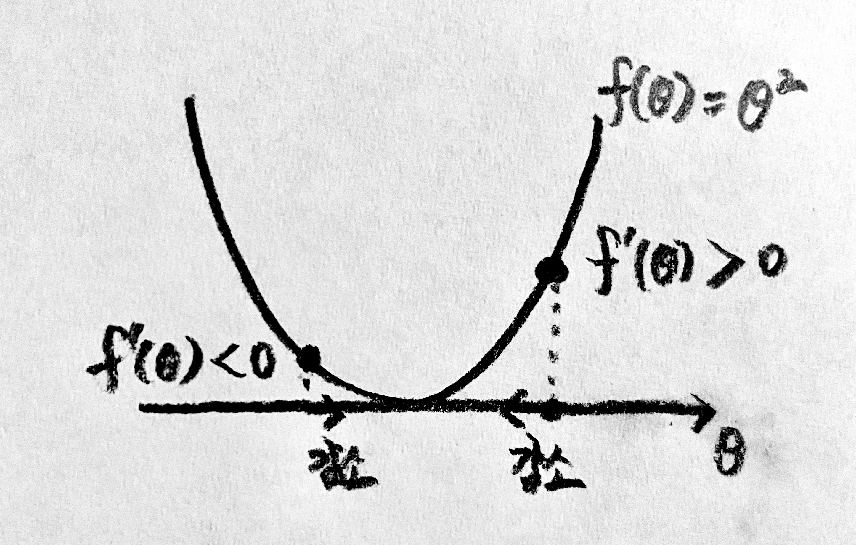
It’s challenging to search for points where $f’(\theta) = 0$ across the entire range of real numbers, but it’s fairly easy to calculate $f’(\theta)$ at a particular point and check its sign. If so, it seems like it’s good idea to slightly decrease $\theta$ whenever $f’(\theta)$ is greater than $0$. Similarly, let’s slightly increase $\theta$ whenever $f’(\theta)$ is less than $0$. If we continue this process, $f(\theta)$ will keep decreasing.

The process can be expressed with the following equation:

\[\begin{equation}\theta^{(k+1)}=\theta^{(k)}-\alpha\:\text{sgn}\:f'(\theta^{(k)})\end{equation}\]

In this, $\alpha$ is a sufficiently small positive number. The notation $\text{sgn} \;\cdot$ represents the sign of $\cdot$.⁴ Also, $\theta^{(k)}$ denotes the value of $\theta$ at the $k$-th step. If our intuition is correct, the real variable $\theta$ starts from its initial value $\theta^{(0)}$ at the very first step, $k=0$, and gradually approaches the minimum point according to the above recurrence relation. Specifically, unless $f(\theta)$ is an unusual function, $\theta$ will approach the global minimum point of $f(\theta)$, which is $\theta=0$. Let’s verify that as the value of $k$ increases, $\theta^{(k)}$ generally decreases.

However, there’s a problem with the above approach. The magnitude of $\alpha\:\text{sgn}\:f’(\theta^{(k)})$,

\[\begin{equation} \left|\alpha\:\text{sgn}\:f'(\theta^{(k)})\right|=\left|\alpha \cdot(\pm1)\right| \end{equation}\]

is always $\alpha$. This means that even when approaching the minimum value, $\theta^{(k)}$ is updated only by a fixed step-size of $\alpha$. In other words, if we only consider the sign, we won’t converge to the minimum value and will instead be oscillating by a magnitude of $\alpha$! Therefore, we should gradually decelerate as we approach the exact minimum value.

On the other hand, we can know when we’re close to the minimum value by noticing that the magnitude of $\lvert f’(\theta)\rvert$ has decreased, i.e., $f’(\theta)$ is close to $0$. Can we use this information to improve the equation? In fact, since $f’(\theta^{(k)})$ is already a real number with a sign, there’s no need to use the $\text{sgn}$ function. Removing the $\text{sgn}$ function gives:

\[\begin{equation} \theta^{(k+1)}=\theta^{(k)}-\alpha f'(\theta^{(k)})\end{equation}\]

This equation addresses the issue in the previous equation where the step-size was fixed at $\alpha$. As $\theta^{(k)}$ approaches the minimum value, the magnitude (absolute value) of $f’(\theta^{(k)})$ decreases, which means that we’ll be decelerating. The direction of movement will remains the same as before, reducing the value of $f$. Thus, it seems all the previous issues have been resolved. The method of optimizing a function as in the above equation is called Gradient Descent (GD).

Surprisingly, for simple functions like $f(\theta)=\theta^2$ we can use concepts of sequences and differentiation learned in high school to determine and prove the conditions under which $\theta^{(k)}$ converges to the state $\theta=0$, the minimum point. Let’s assume $\alpha=0.01$ and start from $\theta^{(0)}=1$. Since $f’(\theta)=2\theta$, substituting this into the original equation gives:

\[\begin{align} \theta^{(k+1)}&=\theta^{(k)}-0.02\:\theta^{(k)}=0.98\:\theta^{(k)},\newline \theta^{(k)}&=0.98^k \theta^{(0)}=0.98^k. \end{align}\]

Since $0<0.98<1$, the sequence $\theta^{(k)}$ converges to $0$ as $k$ approaches infinity.

\[\begin{equation} \theta^{(k)}=0.98^k \rightarrow 0 \;\;\text{as}\;\; k\rightarrow \infty. \end{equation}\]

However, if the magnitude of $\alpha$ is too large, the sequence $\theta^{(k)}$ might diverge! For instance, if $\alpha=2$ and we start from $\theta^{(0)}=1$ as before:

\[\begin{equation} \begin{aligned} \theta^{(k+1)}&=\theta^{(k)}-4\:\theta^{(k)}=(-3)\,\theta^{(k)}, \newline \theta^{(k)}&=(-3)^k, \newline \theta^{(0)}&=(-3)^k. \end{aligned} \end{equation}\]

In this case, the sequence $\theta^{(k)}$ oscillates and diverges as $k$ approaches infinity.

\[\begin{equation} \theta^{(k)}=(-3)^k \text{ oscillates as } k\rightarrow \infty. \end{equation}\]

Check Problem 1.

When applying gradient descent to the function $f(\theta) = \theta^2$, what are the conditions for $\alpha$ and $\theta^{(0)}$ for $\theta^{(k)}$ to converge to the optimal solution $\theta = 0$? Note that $\alpha > 0$.

• Answer $0<\alpha<1$ or $\theta^{(0)}=0.$

Coding Problem 1.

Let’s apply gradient descent to the function $f(\theta) = (\theta + 3)^2$. Specifically, with a learning rate of $\alpha = 0.7$ and starting from the condition $\theta^{(0)} = -4$, update the value of $\theta$ according to equation $(4)$. List the values of $\theta$ from $\theta^{(0)}$ to $\theta^{(30)}$ and use the print() function to display them.

• Answer

  # Code
  
  alpha = 0.7
  theta = -4
  thetas = []               # Create an empty list
  thetas.append(theta)      # Save initial theta
  for i in range(30):
      theta = theta - alpha * (2 * (theta + 3))  # Apply gradient descent
      thetas.append(theta)
  print(thetas)             # Print values for theta
  

  # Output
  
  [-4, -2.6, -3.16, -2.936, -3.0256, -2.98976, -3.004096, -2.9983616, -3.00065536, -2.999737856, -3.0001048576000002, -2.9999580569599997, -3.000016777216, -2.9999932891136, -3.00000268435456, -2.999998926258176, -3.0000004294967297, -2.9999998282013083, -3.0000000687194768, -2.9999999725122093, -3.0000000109951164, -2.9999999956019536, -3.0000000017592185, -2.9999999992963127, -3.000000000281475, -2.99999999988741, -3.000000000045036, -2.9999999999819855, -3.000000000007206, -2.999999999997118, -3.000000000001153]
  

Local Minima and Global Minima

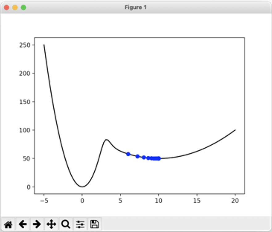
The local minimum point of a function $f(\theta)$, denoted as $\theta_\text{local}$, is a point where the function value is less than or equal to the values in the neighborhood⁵ of $\theta$, i.e., $f(\theta)\ge f(\theta_\text{local})$ for $\theta$ in the neighborhood of $\theta_\text{local}$. In the graph of the univariate real function $f$ above, with the horizontal axis as the $\theta$-axis, the points $\theta=0$ and $\theta=10$ are local minima points because their function values are always less than those of their neighboring points. The function value at a minimum point is called the minimum value. Thus, the function $f$ has a local minimum value of $f(0)=0$ at $\theta=0$ and a local minimum value of $f(10)=50$ at $\theta=10$.

On the other hand, the global minimum point of the function $f(\theta)$, denoted as $\theta_\text{global}$, is a point where the function value is less than or equal to the values at all points in its domain, i.e., $f(\theta)\ge f(\theta_\text{global})$ for all $\theta$ within the domain of $f$. In the above case, $\theta=0$ is both a local and global minimum, but $\theta=10$ is only a local minimum. This is because the function value at $\theta=0$, which is $f(0)=0$, is less than the function value at $\theta=10$, which is $f(10)=50$.

When we applied the gradient descent method to the function $f(\theta)=\theta^2$, we observed that if $\alpha$ is sufficiently small, the sequence $\theta^{(k)}$ converges well to the optimal solution $\theta=0$. However, for $f(\theta)=\theta^2$, as there’s only one local minimum (and because the function values shoot to $\infty$ as $\theta$ approaches $\pm \infty$), the local minimum is the same as the global minimum. But for functions like $f$ in the above graph with multiple local minima, it’s uncertain whether $\theta$ will converge to the global minimum, as it can get stuck in a minimum that is local but not global.

For instance, in some cases, a company’s profit structure might be hard to improve with minor adjustments. If any slight modification to the current structure only worsens profitability, the company might need to completely overhaul its structure to expect significant profit growth. This can be interpreted as an effort to escape from a local minimum. Another example is misconceptions during learning. Even with misconceptions, one might still be able to explain phenomena adequately. However, as one encounters more information, it’s more effective to break away from the misconception and relearn, enhancing the ability to explain phenomena. In other words, it’s preferable to move away from the misconception (local minimum) and relearn a more accurate concept (global minimum).

While gradient descent ensures convergence to a local minimum under appropriate assumptions, it doesn’t guarantee convergence to a global minimum.⁶ Hence, optimization algorithms like Momentum and Adam, which include inertial terms to escape shallow local minima and head towards deeper global minima with smaller function values, have been developed. If you’re interested in exploring various optimization techniques like Momentum and Adam, consider checking out the referenced post below after reading Part II of this series.

A Comprehensive Guide on Optimizers in Deep Learning

Check Problem 2.

For the quartic function $f(\theta) = \theta^2(\theta-1)(\theta-2)$:

(a) Find the local minimum point.

(b) Find the global minimum point.

(c) Determine the minimum value at the point which is a local minimum but not a global minimum.

• Answer (a) local minimum point: $\theta=0,\;\theta=\frac{9+\sqrt{17}}{8}\approx1.640$ (b) global minimum point: $\theta =\frac{9+\sqrt{17}}{8}\approx1.640$ (c) $f(0)=0$

Coding Problem 2.

Let’s apply the gradient descent method to the quartic function $f(\theta) = \theta^2(\theta-1)(\theta-2)$.

(a) With a learning rate of $\alpha = 0.05$ and starting from $\theta^{(0)} = 3$, update the value of $\theta$ using equation $(4)$. List the values of $\theta$ from $\theta^{(0)}$ to $\theta^{(30)}$ and print them using the print() function.

(b) Check if $\theta$ converges to the global minimum. If it does, find the convergence value of $f(\theta^{(k)})$.

(c) Identify one initial value of $\theta^{(0)}$ for which $\theta$ does not converge to the global minimum. Note that $\alpha = 0.05$.

• Answer (a)

  # Code
  
  alpha = 0.05
  theta = 3
  thetas = []               # Create empty list
  thetas.append(theta)      # Save initial theta
  for i in range(30):
      # Gradient descent
      theta = theta - alpha * (4 * theta**3 - 9 * theta**2 + 4 * theta)
      thetas.append(theta)
  print(thetas)             # Print values of theta
  

  # 출력값
  
  [3, 1.0499999999999998, 1.1045999999999998, 1.1631899369327998, 1.2246451065084327, 1.2872724414731267, 1.3488794094514513, 1.4070169240305987, 1.4593836892273668, 1.5042779940878397, 1.540914144056721, 1.5694643322257227, 1.5908330465698923, 1.6063037620026415, 1.6172175322689708, 1.6247689357696435, 1.629921406541151, 1.6334027143439558, 1.6357390290643616, 1.6372997348435627, 1.6383390867159184, 1.6390298045931315, 1.6394881953333464, 1.6397921226262633, 1.6399935122140699, 1.640126903506169, 1.6402152319777135, 1.6402737104854812, 1.6403124220218963, 1.6403380462312662, 1.640355006705482]
  

  (b) We can observe that theta is converging to the global minimum point 1.640. To evaluate the function at this point:

  # Code
  
  theta_global = thetas[30]  # Assume the 30th theta is sufficiently close to the global minimum point
  print(theta_global**2 * (theta_global - 1) * (theta_global - 2))
  

  # Output
  
  -0.6196843457001793
  

  (c) If we run the code with $\theta^{(0)}=-1$,

  # Output
  
  [-1, -0.1499999999999999, -0.10919999999999994, -0.08173347786239996, -0.06227141782417553, -0.0480238616518109, -0.037359106839121914, -0.029248790740098913, -0.023009056880295777, -0.018166571714116383, -0.01438354734163941, -0.011413143825789467, -0.00907160079235181, -0.0072200990529043794, -0.0057525455421655915, -0.004587107060241312, -0.0036601976461915, -0.002922119638721227, -0.0023338482682754252, -0.001864624990714408, -0.0014901341241158653, -0.0011911074126556803, -0.0009522471605601266, -0.0007613895071587255, -0.0006088506461576267, -0.00048691365718682596, -0.00038942421445218494, -0.00031147111670195584, -0.0002491332309026941, -0.00019927865131451355, -0.00015940504907746946]
  

  We can observe that theta is converging to the point $\theta=0$ (which is a local minimum point, but not a global minimum point)

---